Python — Hello World Machine Learning!

In this blog, I will cover the various Machine Learning algorithm’s model building and predict the accuracy of each model using the Python popular scientific libraries (scipy, numpy, matplotlib, pandas, sklearn).

This is a very good sample hello world example to get started with Machine Learning using Python!

Used iris flowers dataset to build the models and predict the accuracy. This dataset is called as “hello world” dataset in machine learning and statistics!

Refer here for Iris dataset information https://archive.ics.uci.edu/ml/machine-learning-databases/iris/iris.names

From the above link, you understand that dataset has 4 input attributes and 1 output attribute i.e.

Attributes

:

 — sepal length in cm

 — sepal width in cm

 — petal length in cm

 — petal width in cm

Classes

:

 — Iris Setosa

 — Iris Versicolour

 — Iris Virginica

Source code for this blog can be found here [GitHub — Jayasagar/python-machine-learning-hello-world]( https://github.com/Jayasagar/python-machine-learning-hello-world )

What’s covered?

• Prerequisites

• Basic concepts to understand

• Load Dataset

• Data Statistics, Summary and its Visualization

• Experiment with various Algorithms

• ** Split ‘train and test’ validation subsets

• ** Learn cross-validation Result (Build various models)

• ** Predict accuracy of the model on the validation dataset

• ** Repeat the above two steps for other Algorithms

• ** Plot cross-validation accuracy of all the models

• Finally!

Prerequisites

I will assume you have little Python experience and below listed concepts.

Basic concepts to understand

Apart from knowing the language and libraries(NumPy, Pandas, matplotlib, sklearn), it would be great to understand certain basic concepts so that it really helps to understand what and why we do!

Note: There are quite many basics and keywords to understand in total, below list is some of them required for this tutorial!

• Input attribute/Feature

• Output class category

• Model

• Dataset

• Training dataset

• Gaussian/Normal distribution

• Validation/Test dataset

• Box plot ::

• Scatterplot matrices

• Prediction

• Maths (Mean, Variance, Standard Deviation, etc…)

• Cross-Validation: Quick intro read

• Confusion Matrix: Quick intro read

Load Dataset

You can use one of the following approaches to load iris dataset!

Load using sklearn.datasets

from sklearn import datasets

# Load the iris data set sklearn

def

loadPreBuiltIrisDataset

():

return

datasets

.

load_iris()

Load from project

import pandas

as

pd

# read training set data from the CSV format

def

getTrainingDataset

():

trainingDataset

=

[]

inputAttributes

=

['sepal-length', 'sepal-width', 'petal-length', 'petal-width', 'class']

dataset

=

pd

.

read_csv('iris.data.txt', names

=

inputAttributes)

# print('my_dataframe.columns.values.tolist()', list(df))

numpyMatrix

=

dataset

.

as_matrix()

#print('at index dataframe:', df[0])

print

('NumPy Dataset Array using Pandas', numpyMatrix)

return

numpyMatrix

Load from remote url

def

loadDatasetFromUrl

():

url

=

"

https://archive.ics.uci.edu/ml/machine-learning-databases/iris/iris.data

"

names

=

['sepal-length', 'sepal-width', 'petal-length', 'petal-width', 'class']

return

pd

.

read_csv(url, names

=

names)

You can load the dataset in various ways from remote URL, download the iris dataset or load using sklearn. Three ways covered in the above code examples.

Data Statistics, Summary and Visualization

It is always good to start with quick information to get a basic understanding of the data, such as,

• Matrix dataset shape(No of dimensions, row and column length in each dimension)

• Statistical Summary(count, mean, min, max, etc…)

• Output class distribution

• Graph data visualizations

Here, we will try to see each one of the above points

Shape

# Shape

shape

=

dataset

.

shape

print

('Shape:', shape)

print

('Number of Dimensions:', len(shape))

#Output

#shape: (150, 5)

#Number of Dimensions: 2

In the above code example, the result (150, 5), is the tuple object and its length is 2 i.e. number of dimensions! Each value in tuple indicates the length of the data size in each dimension(150 and 5).

Statistical Summary

I really like the describe method call as it gives a very good summary on each input attribute/feature!

# Statistical Summary(count, mean, min,max, etc…)

print

(dataset

.

describe())

sepal-length sepal-width petal-length petal-width count 150.000000 150.000000 150.000000 150.000000 mean 5.843333 3.054000 3.758667 1.198667 std 0.828066 0.433594 1.764420 0.763161 min 4.300000 2.000000 1.000000 0.100000 25% 5.100000 2.800000 1.600000 0.300000 50% 5.800000 3.000000 4.350000 1.300000 75% 6.400000 3.300000 5.100000 1.800000 max 7.900000 4.400000 6.900000 2.500000

Output class distribution

# Output class distribution

print

(dataset

.

groupby('class')

.

size())

Iris-setosa 50 Iris-versicolor 50 Iris-virginica 50

Output Class Distribution: 33.3% for each of 3 classes.

Univariate plots

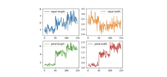
As the name suggests, easy to understand and no confusion with this plotting, it is used for one-variable-at-a-time plots!

import pandas

as

pd

import matplotlib.pyplot

as

plt

# Univariate plots

# subplots=True: Make separate subplots for each column

# layout=(2, 2): (rows, columns) for the layout of subplots

dataset

.

plot(kind

=

'line', subplots

=

True, layout

=

(2, 2), sharex

=

False, sharey

=

False)

plt

.

show()

If you replace ‘line’ with ‘box’ in the above code snippet you see box plotting, which gives a very good idea on data how it’s distributed(minimum, first quartile, median, third quartile, maximum.)

If you replace ‘line’ with ‘box’ in the above code snippet you see box plotting, which gives very good idea on data how it’s distributed(minimum, first quartile, median, third quartile, maximum.)

Histogram Plots

import pandas

as

pd

import matplotlib.pyplot

as

plt

# Histogram Plot

dataset

.

hist()

plt

.

show()

Multivariate Plots

It is used to visualize the relationship between the multiple input attributes! Here we use Scatterplot matrices to view the multivariate plot.

Scatterplot matrices are a great way to roughly determine if you have a linear correlation between multiple variables. This is particularly helpful in pinpointing specific variables that might have similar correlations to your genomic or proteomic data.

Source: [Scatterplot MatricesR-bloggers]( https://www.r-bloggers.com/scatterplot-matrices/ )

By this time, I hope you would have learned some basic insights on data and its visualizations!

Now it's the time to move on with various Machine Learning algorithm’s model building and predict the accuracy of each one. Let’s start!

Experiment through various Algorithms

Before trying out different algorithms, first, let’s define steps we follow

1. Split ‘train and test’ validation subsets

2. Learn cross-validation result(Build various models)

3. Predict accuracy of the model on the validation dataset

4. Repeat the same steps for other Algorithms

5. Plot cross-validation accuracy of all the models

Split ‘train and test’ validation subsets

With the help of model_selection from sklearn package, split the actual dataset into * Train dataset * Test/Validation dataset

In the below code, 20% of the total dataset will be used later for validating the particular algorithm to decide it’s accuracy.

from sklearn import model_selection

X

=

dataset

.

values[:, 0:4]

# Slice Input attribute value from 0 to 3 index

Y

=

dataset

.

values[:, 4]

# Slice Output attribute values

# Split both input/output attribute arrays into random train and test subsets

X_train, X_validation, Y_train, Y_validation

=

model_selection

.

train_test_split(X, Y, test_size

=

0.20)

Read here for more information on train and test data split sklearn.model_selection.train_test_split — scikit-learn 0.19.1 documentation

In the above code, two training sets X_train is the input features/attribute set, Y_train is the output category dataset. Same holds for other two X_validation and Y_validation but it is tested dat i.e. test data for input features/attribute set and output category dataset respectively!

Now, you know how to split the original dataset into two subsets(training and test data)!

Learn cross-validation result (Build various models)

The goal is to identify the best-fit model, we should pick and evaluate some algorithms, in this example below are the algorithms going to be tested and pick one as a best mode fit algorithm!

• Decision Tree Classifier

• Support Vector Machines

• K-Nearest Neighbors

• Logistic Regression

• Linear Discriminant Analysis

• Gaussian Naive Bayes

Linear algorithms(Logistic Regression and Linear Discriminant Analysis)

Nonlinear algorithms (K-Nearest Neighbors, Decision Tree Classifier, Gaussian Naive Bayes and Support Vector Machines).

To understand the steps, instead of evaluating all together rather we pick and evaluate DecisionTreeClassifier(CART), and display its cross-validation accuracy score.

from sklearn.metrics import classification_report

from sklearn.metrics import accuracy_score

from sklearn.tree import DecisionTreeClassifier

# DecisionTreeClassifier Cross validation Result

kfold

=

model_selection

.

KFold(n_splits

=

10, random_state

=

7)

cv_results

=

model_selection

.

cross_val_score(DecisionTreeClassifier(), X_train, y_train, cv

=

kfold, scoring

=

'accuracy')

result

=

"CR Result -> DecisionTreeClassifier: %f (%f)"

%

(cv_results

.

mean(), cv_results

.

std())

print

(result)

Important thing to notice is model_selection.cross_val_score which returns the cross-validation accuracy score.

Output

CR Result -> DecisionTreeClassifier: 0.950000 (0.066667)

Now we have accuracy score ‘0.950000’ for DecisionTreeClassifier algorithm, using K-Fold cross-validation technique.

Above logic has to be repeated for all the algorithms to get their accuracy score.

Predict the accuracy of the model on validation dataset(DecisionTreeClassifier)

In one of the above section ‘Split train and test validation subsets’, we created 20% of the validation test data. Basically, calculate the accuracy of the model using that validation test data.

from sklearn.metrics import confusion_matrix

from sklearn.metrics import classification_report

from sklearn.metrics import accuracy_score

from sklearn.tree import DecisionTreeClassifier

cart

=

DecisionTreeClassifier()

cart

.

fit(X_train, y_train)

#Input Sttribute dataset and Class dataset

predictions

=

cart

.

predict(X_validation)

print

('Accuracy score:', accuracy_score(y_validation, predictions))

print

('Confusion Matrix', confusion_matrix(y_validation, predictions))

print

('Classification report', classification_report(y_validation, predictions))

Output

Accuracy score: 0.966666666667 Confusion Matrix [[10 0 0] [ 0 11 2] [ 0 0 7]]

Classification report

https://medium.com/media/f95122c7872e310d3f5ad88dd3a7dce5/href

From the two outputs, the cross-validation technique shows an accuracy score is ‘ 0.950000’ and Average accuracy score from validation test dataset is ‘0.9666’. Not much difference in the score right!

Repeat the same steps for other Algorithms

In the above two sections, we have seen the accuracy score calculations only for DecisionTreeClassifier. Let’s generalize and reuse the logic to repeat the above two steps to have all results.

Source code can be found @

GitHub — Jayasagar/python-machine-learning-hello-world

from sklearn import model_selection

from sklearn.metrics import classification_report

from sklearn.metrics import confusion_matrix

from sklearn.metrics import accuracy_score

# Helper function to display the Cross Verification accuracy result

def

buildModel

(X_train, y_train, algorithm, model):

kfold

=

model_selection

.

KFold(n_splits

=

10, random_state

=

7)

cv_results

=

model_selection

.

cross_val_score(model, X_train, y_train, cv

=

kfold,

scoring

=

'accuracy')

print

('cv_results:', cv_results)

result

=

"Cross Verification Result -> %s: %f (%f)"

%

(algorithm, cv_results

.

mean(), cv_results

.

std())

print

(result)

return

cv_results

# Helper function to display the accuracy against validation dataset

def

predict

(X_train, X_validation, y_train, y_validation, algorithm, model):

# Prediction Report

model

.

fit(X_train, y_train)

predictions

=

model

.

predict(X_validation)

print

('Accuracy score:', algorithm, accuracy_score(y_validation, predictions))

print

('Confusion Matrix', confusion_matrix(y_validation, predictions))

print

('Classification report \n', algorithm, classification_report(y_validation, predictions))

#Iterate through all the Algorithms and cross verify with test dataset

algorithm_dict

=

{

'CART': DecisionTreeClassifier(),

'NB': GaussianNB(),

'SVC': SVC(),

'K-N': KNeighborsClassifier(),

'LR': LogisticRegression(),

'LDA': LinearDiscriminantAnalysis()

}

results

=

[]

for

key, value

in

algorithm_dict

.

items():

# Learn Cross Validation accuracy result (Build various models)

result

=

buildModel(X_train, Y_train, key, value)

results

.

append(result)

# Predict accuracy of the model on validation dataset

predict(X_train, X_validation, Y_train, Y_validation, key, value)

Plot cross-validation accuracy of all the models

To visualize the cross-validation accuracy of all the models, we can use the box plot.

# Compare Accuracy Results

fig

=

plt

.

figure()

fig

.

suptitle('Models Comparison')

plt

.

boxplot(results, labels

=

algorithm_dict

.

keys(), showmeans

=

True, meanline

=

True)

plt

.

show()

Final results

In the above example, for each algorithm, we evaluated model accuracy is tested two ways, one using cross verification technique and other using the validation subset split from original training data.

Covered in-detail steps to build the first hello world machine learning example using Python!

It is not very hard to make good progress if you know little Python and understand a few fundamental math and Python libraries.

I hope you learned something from this! Thank you for reading. Feedback is much appreciated.

Python — Hello World Machine Learning! was originally published in tech.at.core on Medium, where people are continuing the conversation by highlighting and responding to this story.